Spatial interpolation
Page contents
Spatial interpolation#
Grid interpolation#
For enhanced visuals, hyoga supports interpolating and remasking model output onto a different (usually higher-resolution) topography. This produces an image which deviates somewhat from the model results, but with detail potentially improving readability.
A necessary first step in many cases is to compute the bedrock deformation due to isostatic adjustment. If the dataset was produced by a model including bedrock deformation, there will be a systematic offset between the model bedrock topography and the new topography onto which data are interpolated.
Warning
Assigning isostasy is not strictly necessary for interpolation to succeed, but omitting it would produce errors in the new ice mask. Of course, it can be safely omitted if the model run does not include isostasy.
In this case, we compute the bedrock deformation by comparing bedrock altitude in the dataset with bedrock altitude in the initial state:
ds = hyoga.open.example('pism.alps.out.2d.nc')
ds = ds.hyoga.assign_isostasy(hyoga.open.example('pism.alps.in.boot.nc'))
The method assign_isostasy() assigns a new variable
(standard name bedrock_altitude_change_due_to_isostatic_adjustment). Next
we run interp()
which interpolates all variables, and recalculates an ice mask based on the new
topographies, corrected for bedrock depression in this case. This uses yet
another demo file, which contains high-resolution topographic data over a small
part of the model domain.
ds = ds.hyoga.interp(hyoga.open.example('pism.alps.vis.refined.nc'))
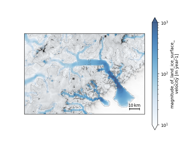
The new dataset can be plotted in the same way as any other hyoga dataset, only with a much higher resolution.
ds.hyoga.plot.bedrock_altitude(center=False)
ds.hyoga.plot.surface_velocity(vmin=1e1, vmax=1e3)
ds.hyoga.plot.surface_altitude_contours()
ds.hyoga.plot.ice_margin(edgecolor='0.25')
ds.hyoga.plot.scale_bar()
Profile interpolation#
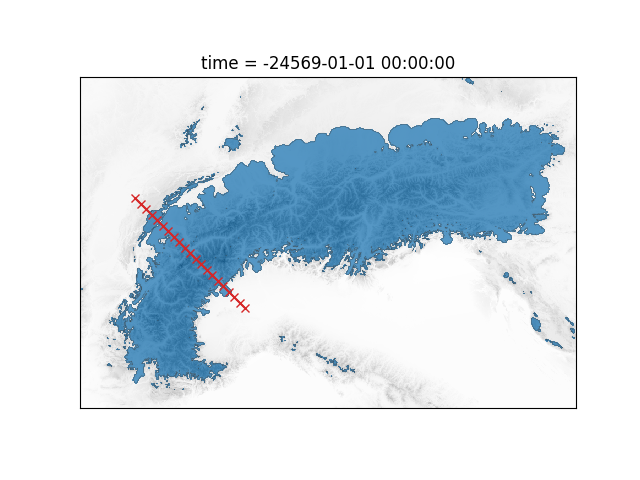
Profile interpolation aggregates variables with two horizontal dimensions (and possibly more dimensions) along a profile curve (or surface) defined by a sequence of (x, y) points. Let us draw a linear cross-section across the example dataset and plot this line on a map.
# prepare a linear profile
import numpy as np
x = np.linspace(250e3, 450e3, 21)
y = np.linspace(5200e3, 5000e3, 21)
points = list(zip(x, y))

# plot profile line on a map
ds = hyoga.open.example('pism.alps.out.2d.nc')
ds.hyoga.plot.bedrock_altitude(center=False)
ds.hyoga.plot.ice_margin(facecolor='tab:blue')
plt.plot(x, y, color='tab:red', marker='x')
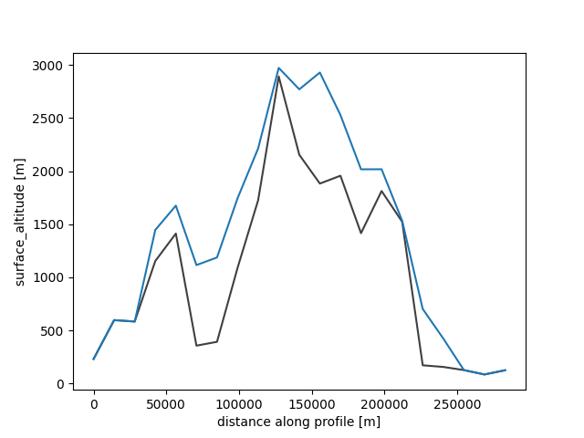
The accessor method profile() can be used to linearly
interpolate the gridded dataset onto these coordinates, producing a new dataset
where the x and y coordinates are swapped for a new coordinate d,
for the distance along the profile.
profile = ds.hyoga.profile(points)
profile.hyoga.getvar('bedrock_altitude').plot(color='0.25')
profile.hyoga.getvar('surface_altitude').plot(color='C0')
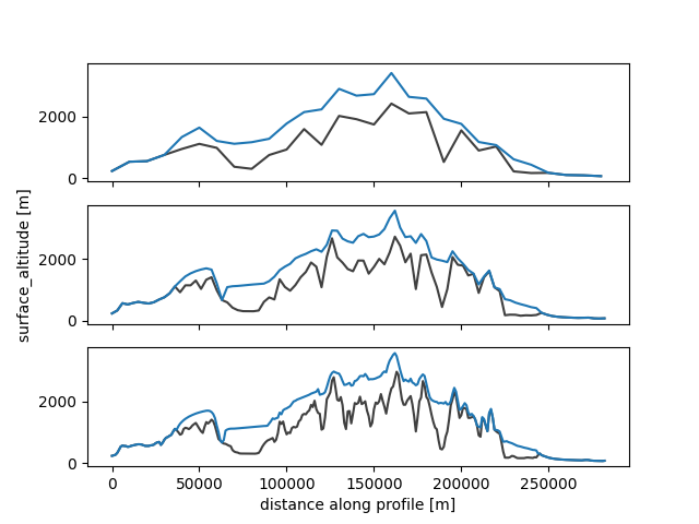
An additional interval keyword can be passed to control the horizontal
resolution of the new profile dataset. This is particularly useful if the
sequence of points is not regularly spaced.
# prepare three subplots
fig, axes = plt.subplots(nrows=3, sharex=True, sharey=True)

# 10, 3, and 1 km resolutions
for ax, interval in zip(axes, [10e3, 3e3, 1e3]):
    profile = ds.hyoga.profile(points, interval=interval)
    profile.hyoga.getvar('bedrock_altitude').plot(ax=ax, color='0.25')
    profile.hyoga.getvar('surface_altitude').plot(ax=ax, color='C0')

# remove duplicate labels
for ax in axes[:2]:
    ax.set_xlabel('')
for ax in axes[::2]:
    ax.set_ylabel('')
The sequence of points in the above example does not have to form a straight
line. Besides, it can also be provided as a numpy.ndarray, a
geopandas.GeoDataFrame, or a path to a vector file containing a
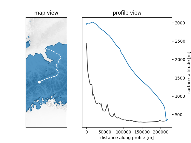
single, linestring geometry. Here is a more advanced example using a custom
shapefile provided in the example data.
#!/usr/bin/env python
# Copyright (c) 2022, Julien Seguinot (juseg.github.io)
# GNU General Public License v3.0+ (https://www.gnu.org/licenses/gpl-3.0.txt)

"""
Profile interpolation
=====================

Demonstrate interpolating two-dimensional model output onto a one-dimensional
profile defined by x and y coordinates inside a shapefile.
"""

import matplotlib.pyplot as plt
import hyoga

# initialize figure
fig, (ax, pfax) = plt.subplots(ncols=2, gridspec_kw=dict(width_ratios=(1, 2)))

# open demo data
with hyoga.open.example('pism.alps.out.2d.nc') as ds:

    # plot 2D model output
    ds.hyoga.plot.bedrock_altitude(ax=ax, center=False)
    ds.hyoga.plot.ice_margin(ax=ax, edgecolor='tab:blue', linewidths=1)
    ds.hyoga.plot.ice_margin(ax=ax, facecolor='tab:blue')

    # interpolate along profile
    ds = ds.hyoga.profile(hyoga.open.example('profile.rhine.shp'))

    # plot profile line in map view
    ax.plot(ds.x, ds.y, color='w', dashes=(2, 1))
    ax.plot(ds.x[0], ds.y[0], 'wo')

    # plot bedrock and surface profiles
    ds.hyoga.getvar('bedrock_altitude').plot(ax=pfax, color='0.25')
    ds.hyoga.getvar('surface_altitude').plot(ax=pfax, color='tab:blue')

# set map axes properties
ax.set_xlim(425e3, 575e3)
ax.set_ylim(5000e3, 5400e3)
ax.set_title('map view')

# set profile axes properties
pfax.set_title('profile view')
pfax.yaxis.set_label_position("right")
pfax.yaxis.tick_right()

# show
plt.show()