Plotting shaded relief
Page contents
Plotting shaded relief#
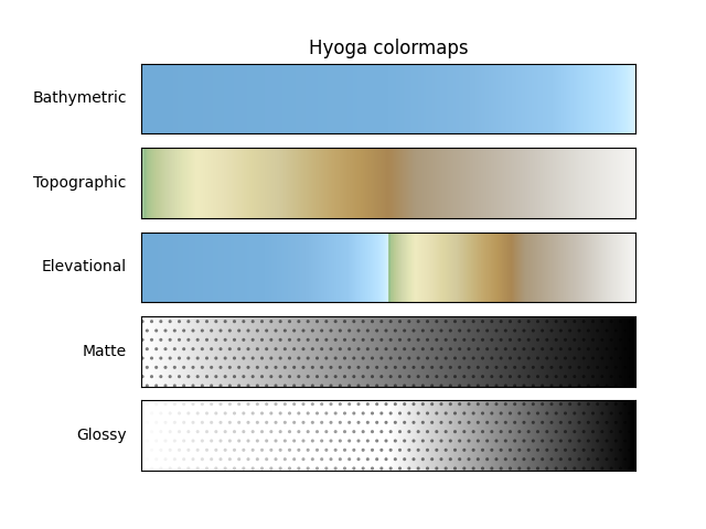
Hyoga colormaps#
In addition to the vast selection of matplotlib built-in colormaps, hyoga
add three custom colormaps for altitude maps (Topographic, Bathymetric,
and Elevational) and two half-transparent colormaps for relief-shading
(Glossy, and Matte).
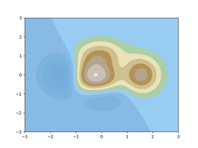
These new colormaps are registered with matplotlib after importing hyoga, which means that they can be used in any matplotlib plot method:
import numpy as np

x = y = np.linspace(-3, 3, 256)
x, y = np.meshgrid(x, y)
z = (1 - x/2 + x**5 + y**3) * np.exp(-x**2 - y**2)
plt.contourf(x, y, z, cmap='Elevational', levels=12)
In addition, these colormaps trigger special behaviour when used in some of
hyoga’s plot methods. Here is an example plotting bedrock altitude contours for
the example data using the Topographic colormap.
with hyoga.open.example('pism.alps.in.boot.nc') as ds:
    ds.hyoga.plot.bedrock_altitude_contours(cmap='Topographic', vmin=0)
    ds.hyoga.plot.bedrock_hillshade(cmap='Glossy')
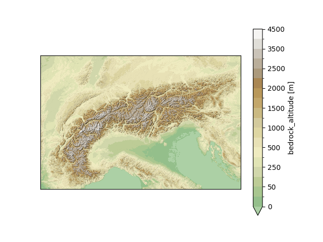
Note how the bedrock altitude contour levels are not equidistant, but are
instead densified at lower elevation to highlight lower reliefs and fit the
highly skewed Topographic colormap.
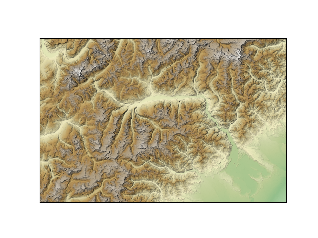
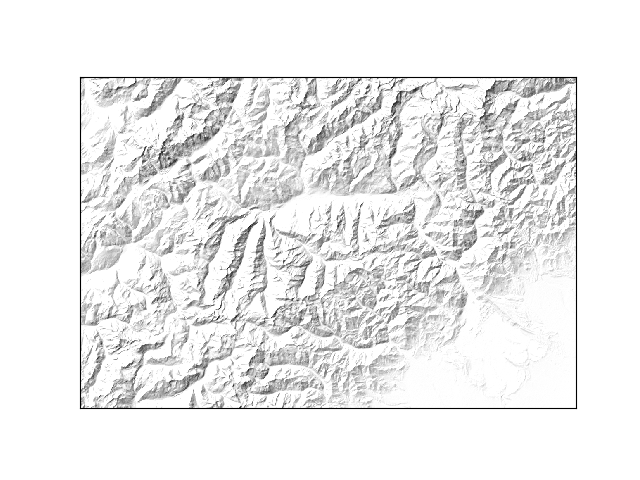
Shaded relief#
Relief shading can be used to add depth to maps. In hyoga, hillshading is
implemented using a slightly differently mechanics than that provided by
matplotlib.colors.LightSource. While matplotlib “blends” hillshades
into topograhic maps, hyoga plots hillshades as a new image independent of
underlying topography. This is what a simple hillshade image looks like:
with hyoga.open.example('pism.alps.vis.refined.nc') as ds:
    ds.hyoga.plot.bedrock_hillshade()
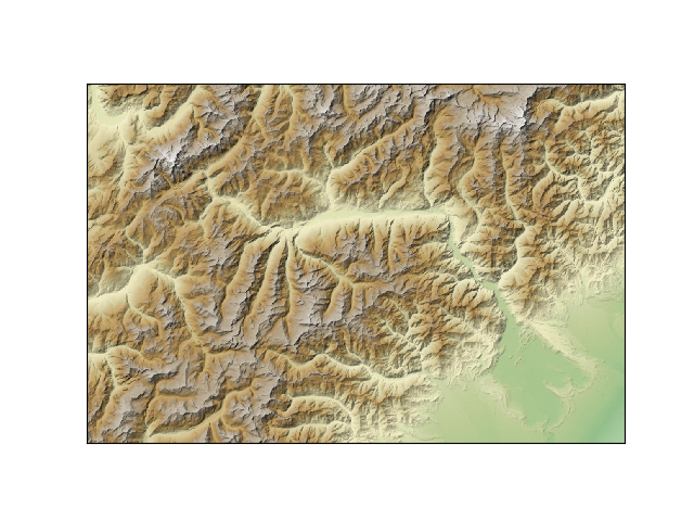
While Dataset.hyoga.plot.bedrock_hillshade() uses the bedrock altitude,
an equivalent Dataset.hyoga.plot.surface_hillshade() plots shaded relief
from the ice surface altitude. By default, however, hillshades are plotted as
a half-transparent layer best overlaid onto an altitude map:
with hyoga.open.example('pism.alps.vis.refined.nc') as ds:
    ds.hyoga.plot.bedrock_altitude(cmap='Topographic')
    ds.hyoga.plot.bedrock_hillshade()
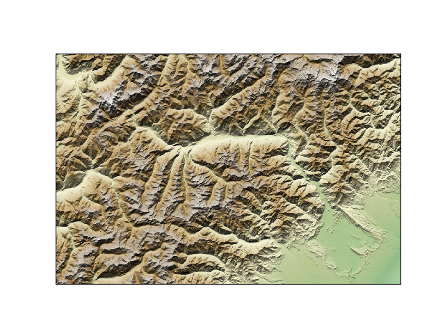
The illumination direction can be customized using altitude and azimuth
angles. Low relief can be accentuated using an exag exaggeration factor:
with hyoga.open.example('pism.alps.vis.refined.nc') as ds:
    ds.hyoga.plot.bedrock_altitude(cmap='Topographic')
    ds.hyoga.plot.bedrock_hillshade(altitude=30, azimuth=-15, exag=3)
The altitude and azimuth arguments accepts lists, allowing
multidirectional shaded relief. The weight arguments applies different
weight to different light sources. The default uses triple illumination from
the northwest. Here is a more advanced example using six weighted light sources
from all directions.
with hyoga.open.example('pism.alps.vis.refined.nc') as ds:
    ds.hyoga.plot.bedrock_altitude(cmap='Topographic')
    ds.hyoga.plot.bedrock_hillshade(
        altitude=45, azimuth=[15, 75, 135, 195, 255, 315],
        weight=[0.2, 0.125, 0.1, 0.125, 0.2, 0.25])