Interpolated streamplot
Note
Click here to download the full example code
Interpolated streamplot#
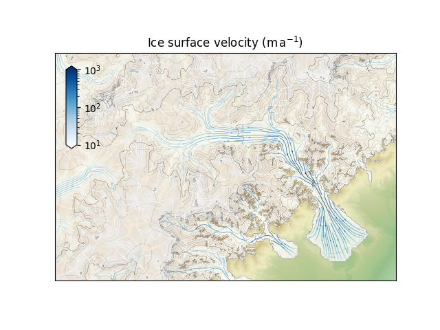
Demonstrate interpolating two-dimensional model output onto a higher-resolution topography provided in a separate file. Bedrock isostatic adjustment needs to be informed in order to correct for the offset between the model and the high-resolution bedrock topographies. This is a rather extreme example with a ten-fold increase in horizontal resolution.
import matplotlib.pyplot as plt
import hyoga

# initialize figure
ax = plt.subplot()
cax = plt.axes([0.15, 0.55, 0.025, 0.25])

# open demo data
with hyoga.open.example('pism.alps.out.2d.nc') as ds:

    # compute isostatic adjustment from a reference input topography
    ds = ds.hyoga.assign_isostasy(hyoga.open.example('pism.alps.in.boot.nc'))

    # perform the actual interpolation
    ds = ds.hyoga.interp(hyoga.open.example('pism.alps.vis.refined.nc'))

    # plot model output
    ds.hyoga.plot.bedrock_altitude(ax=ax, cmap='Topographic', center=False)
    ds.hyoga.plot.surface_altitude_contours(ax=ax)
    ds.hyoga.plot.ice_margin(ax=ax, facecolor='w')

    # plot streamplot
    streams = ds.hyoga.plot.surface_velocity_streamplot(
        ax=ax, cmap='Blues', vmin=1e1, vmax=1e3, density=(6, 4))

    # add colorbar manually
    ax.figure.colorbar(streams.lines, cax=cax, extend='both')

# set title
ax.set_title(r'Ice surface velocity (m$\,$a$^{-1}$)')

# show
plt.show()
Total running time of the script: ( 0 minutes 18.536 seconds)