Natural Earth and GeoPandas
Note
Click here to download the full example code
Natural Earth and GeoPandas#
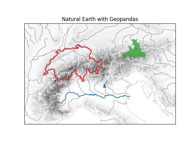
Demonstrate use of GeoPandas to highlight particular Natural Earth features.
downloading https://naturalearth.s3.amazonaws.com/10m_cultural/ne_10m_admin_0_countries.zip...
downloading https://naturalearth.s3.amazonaws.com/10m_cultural/ne_10m_admin_1_states_provinces.zip...
import matplotlib.pyplot as plt
import hyoga


# initialize figure
ax = plt.subplot()

# plot demo bedrock altitude
with hyoga.open.example('pism.alps.out.2d.nc') as ds:
    ds.hyoga.plot.bedrock_altitude(ax=ax, vmin=0)

    # plot canonical Natural Earth background
    ds.hyoga.plot.natural_earth(ax=ax)

    # get dataset crs, we need this
    crs = ds.proj4

# lock axes extent
ax.set_autoscale_on(False)

# plot the Po river and Lago di Garda in blue
rivers = hyoga.open.natural_earth('rivers_lake_centerlines')
rivers[rivers.name == 'Po'].to_crs(crs).plot(ax=ax, edgecolor='tab:blue')
lakes = hyoga.open.natural_earth('lakes')
lakes[lakes.name == 'Lago di Garda'].to_crs(crs).plot(ax=ax)

# plot the outline of Switzerland in red
countries = hyoga.open.natural_earth('admin_0_countries', category='cultural')
countries[countries.NAME == 'Switzerland'].to_crs(crs).plot(
    ax=ax, edgecolor='tab:red', facecolor='none', linewidth=2)

# plot Austria's Salzburg state in green
states = hyoga.open.natural_earth(
    'admin_1_states_provinces', category='cultural')
states[states.name == 'Salzburg'].to_crs(crs).plot(
    ax=ax, alpha=0.75, facecolor='tab:green')

# set title
ax.set_title('Natural Earth with Geopandas')

# show
plt.show()
Total running time of the script: ( 0 minutes 9.235 seconds)