Plotting vector graphics

Hyoga currently supports plotting two types of vector graphics: Natural Earth data data and Last Glacial Maximum Paleoglacier extents. For direct access to geographic vectors see Opening vector data.

Natural Earth data

Natural Earth is a global, public domain geographic dataset featuring both vector and raster data. Only vector data are used in hyoga. Natural Earth vectors are divided in two categories: cultural (countries, populated places, etc) and physical (rivers, lakes, glaciers, etc), and available at three levels of detail referred as the scales 1:10m, 1:50m, and 1:110m.

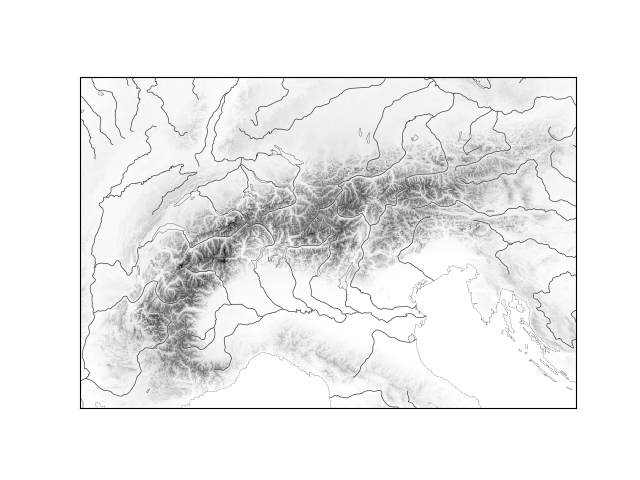
The easiest way to plot Natural Earth as a background for gridded datasets is through the accessor plot method, Dataset.hyoga.plot.natural_earth(). Called without arguments it renders a composite map of rivers, lakes, and the coastline at the highest available scale:

with hyoga.open.example('pism.alps.in.boot.nc') as ds:
   ds.hyoga.plot.bedrock_altitude(vmin=0)
   ds.hyoga.plot.natural_earth()

Warning

To reproject vector data in the gridded dataset projection, a Coordinate Reference System is required. It can be provided in different ways:

• Using decode_coords='all' when opening CF-compliant data with xarray.

• Setting the CRS with rioxarray using Dataset.rio.set_crs().

• In a Dataset.proj4 attribute, as a PROJ string or any other format understood by geopandas.GeoDataFrame.to_crs().

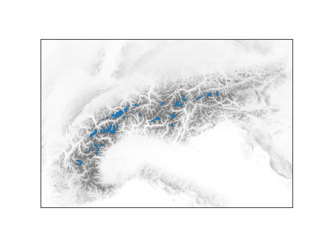
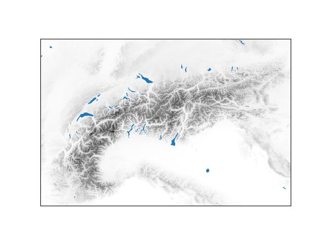
Any other Natural Earth theme from the Natural Earth downloads page can be picked, and the usual matplotlib styling keyword arguments are available. For instance, to plot glaciated areas in blue, use:

with hyoga.open.example('pism.alps.in.boot.nc') as ds:
   ds.hyoga.plot.bedrock_altitude(vmin=0)
   ds.hyoga.plot.natural_earth('glaciated_areas', color='tab:blue')

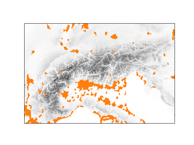
The method defaults to plotting themes in the physical category at the highest scale of 10m. Cultural features require a category='cultural' while lower scales are available through the scale keyword argument:

with hyoga.open.example('pism.alps.in.boot.nc') as ds:
   ds.hyoga.plot.bedrock_altitude(vmin=0)
   ds.hyoga.plot.natural_earth(
       theme='urban_areas', category='cultural', scale='50m',
       color='tab:orange')

Any number of themes can be plotted in a single method call as long as they share the same category and scale:

with hyoga.open.example('pism.alps.in.boot.nc') as ds:
   ds.hyoga.plot.bedrock_altitude(vmin=0)
   ds.hyoga.plot.natural_earth(('lakes', 'lakes_europe'))

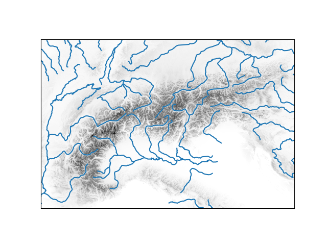
Hyoga also provides two aliases 'lakes_all' and 'rivers_all' that respectively plot, well, all lakes and all rivers at '10m' scale, including such regional subsets as 'lakes_europe'.

with hyoga.open.example('pism.alps.in.boot.nc') as ds:
   ds.hyoga.plot.bedrock_altitude(vmin=0)
   ds.hyoga.plot.natural_earth('rivers_all')

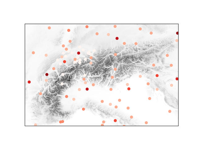
Plotting and reprojection is handled by using geopandas.GeoDataFrame objects in the background, and any additional keywords arguments are passed to geopandas.GeoDataFrame.plot(). This examples plots cities colored by regional significance:

with hyoga.open.example('pism.alps.in.boot.nc') as ds:
   ds.hyoga.plot.bedrock_altitude(vmin=0)
   ds.hyoga.plot.natural_earth(
       'populated_places', category='cultural',
       column='SCALERANK', cmap='Reds_r')

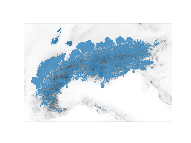
Paleoglacier extents

Paleoglacier extent reconstructions from glacial geology can be used to validate model results or plot standalone maps. The accessor plot method, Dataset.hyoga.plot.paleoglaciers(), will download, cache, re-project and plot paleoglacier extents in the xarray.Dataset coordinates reference system (given by a .proj4 attribute, see Natural Earth data).

with hyoga.open.example('pism.alps.in.boot.nc') as ds:
   ds.hyoga.plot.bedrock_altitude(vmin=0)
   ds.hyoga.plot.paleoglaciers(alpha=0.75)

A source keyword argument controls the source of data plotted, and currently supports two options. The default is a global reconstruction with varying level of accuracy (Ehlers et al., 2011). The alternatively is a more homogeneous but less extensive dataset covering the arctic is and subarctic (Batchelor et al., 2019) accessed by source='bat19'. In either case, only Last Glacial Maximum data are currently supported.

Tip

A consistent, versioned, metadatumed, global datasets of paleoglacier extents would be a huge boost for hyoga. If you know of products even partially fitting this description, please open a Github issue.

Opening vector data

Sometimes more control is needed, or vectors may be plotted independently of gridded data. For such cases, hyoga provides functions to open Natural Earth and paleoglacier vector data for further manipulation.

In the background, accessor plot methods described in previous sections use hyoga.open.natural_earth() and hyoga.open.paleoglaciers() to download, cache, and open vector data as geopandas.GeoDataFrame. The aforementioned (non-plotting) keyword arguments remain available:

hyoga.open.natural_earth(theme='urban_areas', category='cultural')
hyoga.open.paleoglaciers(source='bat19')

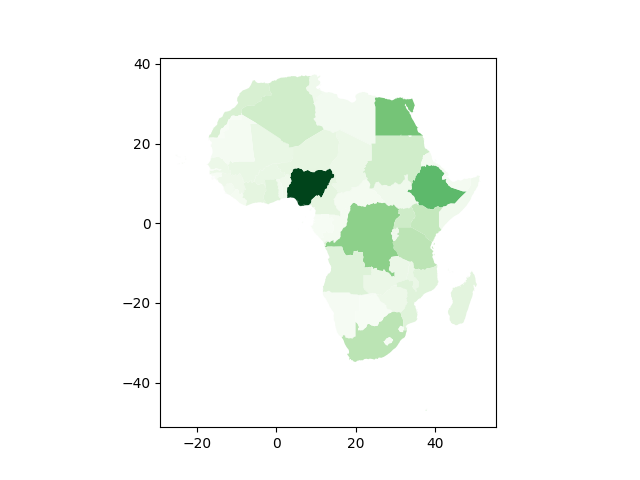
Geodataframes inherit pandas.DataFrame functionality, and thus provide a rich interface to subset, manipulate and visualize geographic vector data. For instance to plot African countries colored by population use:

gdf = hyoga.open.natural_earth('admin_0_countries', category='cultural')
gdf[gdf.CONTINENT == 'Africa'].plot('POP_EST', cmap='Greens')

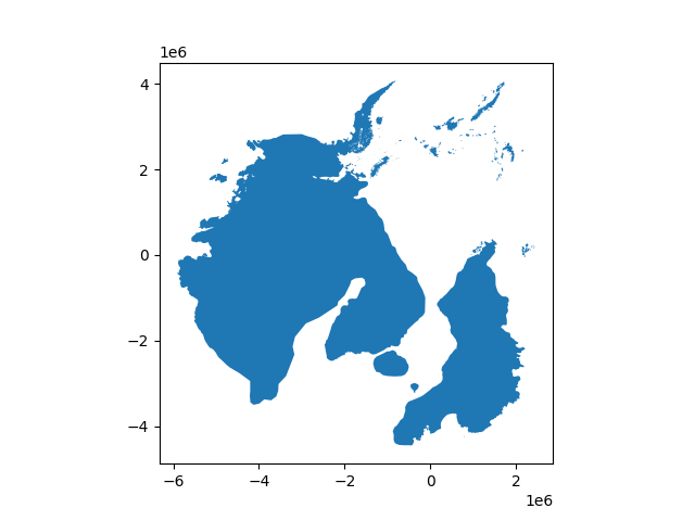
Geodataframes can be re-projected using a variety of coordinate reference system formats. Plotting Batchelor et al. 2019 paleoglacier extents in arctic polar stereographic projection (EPSG 3995) is as simple as:

gdf = hyoga.open.paleoglaciers('bat19')
gdf.to_crs(3995).plot()

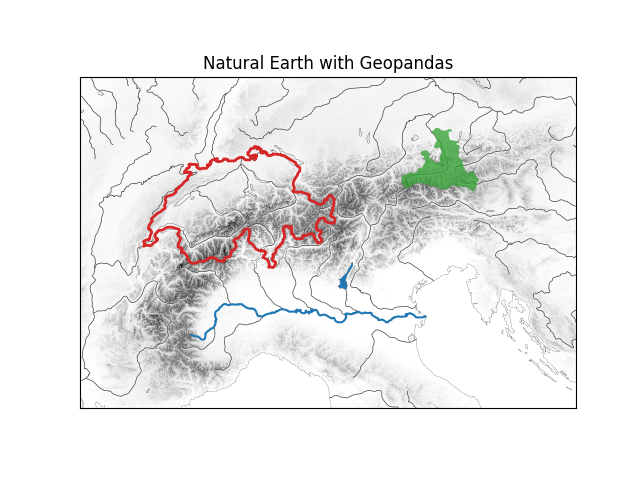
Here is a more advanced example using Natural Earth attribute tables to select particular features within a theme and plot them with a different colour.

#!/usr/bin/env python
# Copyright (c) 2022, Julien Seguinot (juseg.github.io)
# GNU General Public License v3.0+ (https://www.gnu.org/licenses/gpl-3.0.txt)

"""
Natural Earth and GeoPandas
===========================

Demonstrate use of GeoPandas to highlight particular Natural Earth features.
"""

import matplotlib.pyplot as plt
import hyoga


# initialize figure
ax = plt.subplot()

# plot demo bedrock altitude
with hyoga.open.example('pism.alps.out.2d.nc') as ds:
    ds.hyoga.plot.bedrock_altitude(ax=ax, vmin=0)

    # plot canonical Natural Earth background
    ds.hyoga.plot.natural_earth(ax=ax)

    # get dataset crs, we need this
    crs = ds.proj4

# lock axes extent
ax.set_autoscale_on(False)

# plot the Po river and Lago di Garda in blue
rivers = hyoga.open.natural_earth('rivers_lake_centerlines')
rivers[rivers.name == 'Po'].to_crs(crs).plot(ax=ax, edgecolor='tab:blue')
lakes = hyoga.open.natural_earth('lakes')
lakes[lakes.name == 'Lago di Garda'].to_crs(crs).plot(ax=ax)

# plot the outline of Switzerland in red
countries = hyoga.open.natural_earth('admin_0_countries', category='cultural')
countries[countries.NAME == 'Switzerland'].to_crs(crs).plot(
    ax=ax, edgecolor='tab:red', facecolor='none', linewidth=2)

# plot Austria's Salzburg state in green
states = hyoga.open.natural_earth(
    'admin_1_states_provinces', category='cultural')
states[states.name == 'Salzburg'].to_crs(crs).plot(
    ax=ax, alpha=0.75, facecolor='tab:green')

# set title
ax.set_title('Natural Earth with Geopandas')

# show
plt.show()