Plotting glacier data
Page contents
Plotting glacier data#
Plot methods#
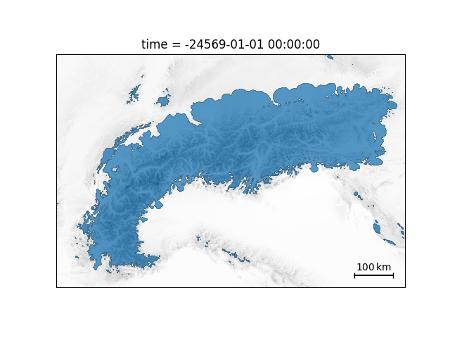
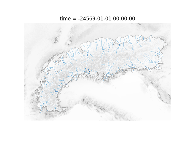
Hyoga include several plot methods that make visualizing ice-sheet modelling datasets a tiny bit more straightforward than using xarray alone. Let’s open an example dataset and plot the bedrock altitude and a simple ice margin contour:
with hyoga.open.example('pism.alps.out.2d.nc') as ds:
    ds.hyoga.plot.bedrock_altitude(center=False)
    ds.hyoga.plot.ice_margin(facecolor='tab:blue')
    ds.hyoga.plot.scale_bar()
Note
Due to isostatic depression, the example bedrock altitude extends slightly
below zero. Here center=False instructs xarray to not center the
colormap around zero despite the negative values. Alternatively, use
vmin and vmax to pass explicit bounds. Use center=True or
center=sealevel in order to plot undersea and land altitudes using a
diverging colormap.
Hyoga alters matplotlib defaults with its own style choices. However, these
choices can always be overridden using matplotlib keyword arguments.
Accessor plot methods such as bedrock_altitude() and
ice_margin() make internal use of
Dataset.hyoga.getvar() to access relevant variables by their
'standard_name' attribute. Here is an example showing variables could
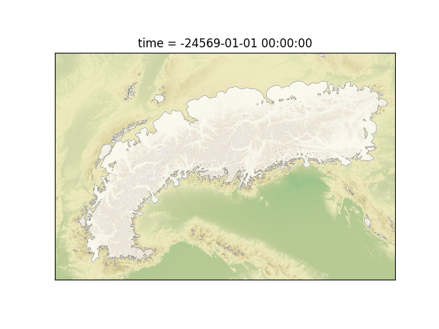
literally be called anything or whatever and still plot:
with hyoga.open.example('pism.alps.out.2d.nc') as ds:
    ds = ds.rename(topg='anything', thk='whatever')
    ds.hyoga.plot.bedrock_altitude(cmap='Topographic', center=False)
    ds.hyoga.plot.ice_margin(facecolor='white')
Inferring variables#
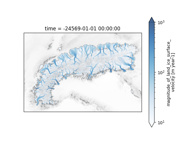
Some missing variables can be reconstructed from others present in the dataset (see Opening datasets). For instance velocity norms are reconstructed from their horizontal components. They plot on a logarithmic scale by default, but the limits can be customized:
with hyoga.open.example('pism.alps.out.2d.nc') as ds:
    ds.hyoga.plot.bedrock_altitude(center=False)
    ds.hyoga.plot.surface_velocity(vmin=1e1, vmax=1e3)
    ds.hyoga.plot.ice_margin(edgecolor='0.25')
Similarly, Dataset.hyoga.plot.surface_velocity_streamplot() accepts a
cmap argument that activates log-colouring of surface velocity streamlines
according to the velocity magnitude:
with hyoga.open.example('pism.alps.out.2d.nc') as ds:
    ds.hyoga.plot.bedrock_altitude(center=False)
    ds.hyoga.plot.ice_margin(facecolor='w')
    ds.hyoga.plot.surface_velocity_streamplot(
        cmap='Blues', vmin=1e1, vmax=1e3, density=(6, 4))
Composite plots#
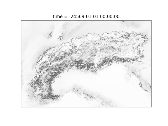
Combining major and minor contour levels at different intervals can be achieved
with a single call to Dataset.hyoga.plot.surface_altitude_contours():
with hyoga.open.example('pism.alps.out.2d.nc') as ds:
    ds.hyoga.plot.bedrock_altitude(center=False)
    ds.hyoga.plot.ice_margin(facecolor='w')
    ds.hyoga.plot.surface_altitude_contours(major=500, minor=100)
More advanced composite examples are available in the Examples gallery.
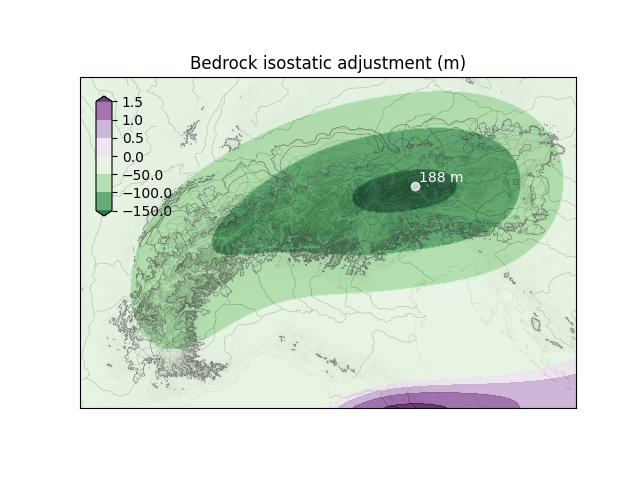
Here is one that uses Dataset.hyoga.assign_isostasy() and
Dataset.hyoga.plot.bedrock_isostasy() to compute and visualize
lithospheric deformation due to the load of the Alpine ice sheet during the
Last Glacial Maximum.
#!/usr/bin/env python
# Copyright (c) 2021-2022, Julien Seguinot (juseg.github.io)
# GNU General Public License v3.0+ (https://www.gnu.org/licenses/gpl-3.0.txt)

"""
Bedrock isostasy
================

Plot a composite map including bedrock altitude, surface altitude contours,
bedroc isostatic adjustment relative to a reference topography in a separate
model input file, and geographic elements.
"""

import matplotlib.pyplot as plt
import hyoga

# initialize figure
ax = plt.subplot()
cax = plt.axes([0.15, 0.55, 0.025, 0.25])

# open demo data
with hyoga.open.example('pism.alps.out.2d.nc') as ds:

    # compute isostasy using separate boot file
    ds = ds.hyoga.assign_isostasy(hyoga.open.example('pism.alps.in.boot.nc'))

    # plot model output
    ds.hyoga.plot.bedrock_altitude(ax=ax, center=False)
    ds.hyoga.plot.surface_altitude_contours(ax=ax)
    ds.hyoga.plot.bedrock_isostasy(
        ax=ax, cbar_ax=cax, levels=[-150, -100, -50, 0, 0.5, 1, 1.5])
    ds.hyoga.plot.ice_margin(ax=ax)

    # add coastline and rivers
    ds.hyoga.plot.natural_earth(ax=ax)

# set axes properties
cax.set_ylabel('')
ax.set_title('Bedrock isostatic adjustment (m)')

# show
plt.show()